E11 Lab #1
2001

Lab report due the next time you come to lab.

Before you start this lab, be sure to read the lab rules.  You may also want to read the guide to BenchLink software.

The room where you will be doing this (and other) labs has computers equipped with web browsers, so you need not print this out (though you certainly may, if you would like to).  Since this document is fairly long, you should look through it at least once before coming to lab.

Introduction to Op Amps and Laboratory Equipment

This laboratory exercise will familiarize you with the equipment you will be using throughout the semester, as well as introducing you to Operational Amplifiers, one of the fundamental building blocks of analog circuitry.  Since there is very little theory involved in this lab, there will not be a formal report.  

The lab exercise is split into four parts

1. Verification of Ohms Law (Use of voltmeters and ammeters)

2. Use of the Oscilloscope and Function Generator

3. Op Amps

4. Finishing up

Verification of Ohms law

1. Connect the circuit shown with R=10kW. Use the resistance boxes, variable DC supplies, and DVM's (Digital Volt-amp-ohm Meters) that are in teh lab.    Note that voltage is measured between two points (across a circuit element), while current is measured through a part of the circuit. For this reason you must always break a circuit to insert an ammeter to measure current.
2. Vary the voltage from 0 to 10 volts in approximately 1 volt increments and record the measured voltage and current at each setting. Then come down again from 10 to 0 volts to check for consistency. There is no reasong to use increments of exactly 1 volt, just be sure to record the voltages carefully.

3. Repeat b with a 20kW resistance.

Use of the Oscilloscope and Function Generator

We will use the oscilloscope to measure voltage waveforms as a function of time.  The function generator creates a wide variety of different voltage waveforms that we will use as inputs to circuits that we build.

The Oscilloscope

Let's examine the HP54602B oscilloscope (or simply "scope") first.

The scope has a display screen on the left and several controls on the right.  By the end of this lab you should know what most of these buttons do.    The controls are split up into 5 separate areas as shown below. 

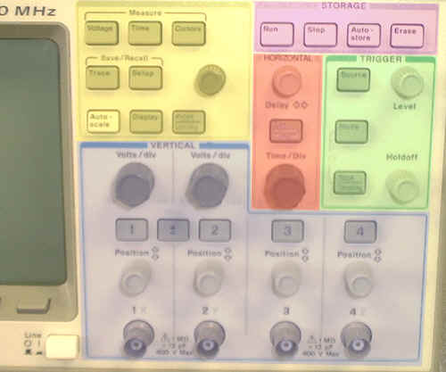
• The largest section (blue - roughly the bottom half of the front panel) is for the inputs, and is labeled "VERTICAL".  The controls in this section set the vertical scale for the voltage waveforms being displayed.  The oscilloscope has four inputs, called channels. In this section of controls each input (there can be up to four) also has a BNC (perhaps for Bayonet Needle Connector, but I've never found a definitive answer) connector, to which the input is connected.  If you look closely at the connector you'll see that there are two conducting (metallic) elements that are electrically shielded from each other.  The inner connector is called the "pin" and is where the voltage signal is applied.  The outer conductor is called the "shell" and is connected to a ground reference.  All of the shells are connected internally, so you needn't connect more than one of them.
• There is another section labeled "HORIZONTAL" (red).  This section is used to set the time scale (or "time base") for the voltage waveform being displayed.
• Next to the "HORIZONTAL" section is one labeled "TRIGGER" (green).   You will learn what this does soon enough. 
• There is a fourth area labeled "STORAGE" that is used, naturally enough, to store waveform data (purple).
• The last section is the one in the upper left that is used for a wide variety of measurement and utility functions (yellow).  We will use these at various times throughout the semester.

The first three sections listed are the most important.

The Function Generator

Shown below is a diagram of the Wavetek Model 20 function generator.   You will learn about the individual controls during the course of the lab.   You should pay special attention to the controls labeled 1, 2, 3, 4, 5, 7, 8 and 9.

 

Use of the Oscilloscope and Function Generator

Turn on the oscilloscope (the "Line" button") and the function generator (the "Power" button).  Connect the "Func Out" output of the function generator to the channel "1" input of the oscilloscope using a BNC cable.  Note that this cable has two conductors (which is needed for a voltage measurement, which is always the difference between two potentials).

All of the information about the most important scope settings is shown on the top of the scope screen.  A typical screen is shown below (from an HP manual).   The information includes which channels are on, and the voltage scale.  Next on the display is information about the time base, followed by information about the triggering mode.  The rightmost label is the "STORAGE" mode.

Setting the "VERTICAL" controls

Make sure that channel 1 is turned on and the others are all turned off.   To turn channel 1 on hit the button labelled "1" in the "VERTICAL" section.  A menu will appear at the bottom of the screen just above the row of six buttons.

• Make sure that the leftmost selection, labelled "1"  is set to "On". 
• Also set "Coupling" to "DC"
• Set "BW Lim" to "Off"
• Set "Invert" to "Off"
• Set "Vernier" to "Off"
• Set "Probe" to "1"
• Turn the Volts/Div knob until the voltage scale (on the top of the screen) reads "500 mV".  This means that each vertical division on the screen represents 500 mV.  So if a signal takes up 4 divisions, it represents a change of 2 volts.

Go to the other three channels, by hitting the corresponding buttons, and turn them off by setting the leftmost selection to "Off". 

Set the function generator as follows:

• Sine wave output (using the buttons labelled "9" in the figure above). 
• Make sure both attenuation buttons (labelled "8") are out
• Set the amplitude ("4") about midway between the minimum and maximum settings
• The DC offset ("3") should be "Off"
• The frequency range knob ("2") should be set to "x1K"
• The frequency select knob ("1") should be set to "1.0"

Setting the triggering as follows (all buttons in the "TRIGGER" area):

• hit the "Source" button and select 1 from the screen menu.  This sets the trigger source as channel 1.  If you had signals connected to the other inputs you could use them as the trigger input.
• Select "Mode" and hit "Auto"
• Select "Slope" and choose from the menu:
  • The upwards pointing arrow
  • DC Coupling
  • Turn REJECTion off

  • Turn Noise Rejection off

Setting the time base ("HORIZONTAL" section)

• change the "Time/Div" (Time per Division) knob until the time is 500 microseconds per division.  The time per division is shown at the top of the screen.   As you change the time base it is highlighted.  Change it until it reads "500 ms/".

• Hit the "Main/Delayed" button and set "Horizontal mode" to "Main", "Vernier" to "Off" and "Time Ref" to "Cntr" (Center).

You should know have a screen that looks something like that shown below.   If you can't get this to work, come see me.  You can get this image from the BenchLink software by choosing Image->New.  Do this now, but first you must initialize the Benchlink Software, if you have not done so yet.  Downloading an image takes a minute or two.

You can get a similar image without some of the detail by choosing Waveform->New.  Try this now.

The advantage of choosing Waveform over Image is that is is quicker and you actually get a series of points representing the waveform data (i.e., voltages versus time).  This means that you can do more with the data after the lab is finished than you can with the image data.

Understanding the function generator.

1. Figure out what the Frequency range knob ("2") and the frequency select knob ("1") do.
2. Figure out what the amplitude ("4") knob does.
3. Figure out what the output select knobs ("9") do.
4. Figure out what the attenuation buttons ("8") do.
5. To understand what the DC offset knob ("3") does, set the function generator to a sine wave output.  The output created by the function generator can now be written:
          V(t)=A+B*sin(w*t)
   This means that the output voltage (V(t)) is equal to a constant signal (A) and a time varying part (B*sin(w*t)).  The constant is called the DC (Direct Current) part of the signal.  The time varying part is calle the AC (Alternating Current).  This is somewhat of a misnomer because all the signals measured by the oscilloscope are voltage, but it is the convention.  By turning the DC offset off, the value of "A" is set to zero.  When you turn the DC offset knob, the signal moves up and down on the scope screen.
6. Experiment with all of these controls to make sure you understand them.

 

Understanding the Oscilloscope.

1. Figure out what the "Volts/Div" knob in the "VERTICAL" section of the front panel does.
2. Figure out what the "Position" knob in the "VERTICAL" section does (note the ground reference shown at the right of the screen).
3. Hit the button labelled "1" in the "VERTICAL" section and figure out what the "Coupling" option on the screen menu does.  Set the function generator so that it has a DC offset (see above) and then set the "Coupling" to "AC".  Then set it to the ground symbol, then set it back to "DC".  Make sure you understand the difference between "AC" and "DC" coupling.  You should be able to explain it in terms of which part of the signal  V(t)=A+B*sin(w*t) is being displayed in each mode.
4. Figure out what the "Time/Div" knob in the "HORIZONTAL" section of the front panel does.
5. Turn the top knob (labeled "Delay") in the "HORIZONTAL" section does.
6. The hardest part of the oscilloscope to understand is triggering.  An oscilloscope is generally (always, in this class) used to display repetitive signals.  In order to have the signal displayed clearly on the screen, consecutive repetitions must be displayed exactly on top of each other.  To do this we pick a point on the wave which we call the trigger point, and place this point at the same place on the screen.  This ensures that consecutive waveforms are displayed one on top of another.  The trigger point is determined by a "level" and a "slope".  The scope is set up now so that the trigger point is in the middle of the screen.
   1. Turn the "Level" knob in the "TRIGGER" area.  Notice how the voltage of the signal at the center of the screen changes to be equal to the trigger level (which is displayed as a horizontal line on the screen as long as you continue to turn the knob).  Note that if you set the trigger level beyond the extrema of the signal being displayed, that you no longer get a nice static display (because the scope must try to decide for itself when to trigger, since the signal never crosses the trigger level).
   2. In addition to the trigger level it is necessary to define the trigger slope, since the waveform crosses each voltage twice -- once while increasing (positive slope) and once while decreasing (negative slope).  This slope is set via the on-screen menu after hitting the "Slope/Coupling" button.  Try it.
7. The last thing you should know is that you can change the location of the trigger point on the screen by hitting the "Main/Delayed" button and changing the "Time Ref" to "Lft" (Left), which moves the trigger point from the center of the screen to the left side.

This obviously only touches upon some of the features of these oscilloscopes.   We'll use a couple of others in the next section, but the features described in the previous section are the only ones that you'll be tested upon.

One last bit of information.  If you are having trouble getting a good picture on the screen, you can always hit the button labelled "Auto-scale" which will try to set all the various modes and scales of the oscilloscope in order to get a good picture.  Though this seems like a wonderful idea, use this feature with caution.   In trying to come up with a good picture, it may set modes that you don't expect (for example, choosing between "AC" and "DC" coupling), so you can easily misinterpret the scope output unless you go back to see how all of the modes are set.

 

Using Op Amps

In this lab, and throughout the semester, you will be using op amps, the basic building blocks of analog electronics. For our purposes we will be using an ideal model of the op amp. The circuit symbol for an op amp is shown.

The op amp obeys the input-output relationship:

v_o=A(v⁺ - v^-)

where v_o is the output voltage, v⁺ and v^- are, respectively, the voltages at the non-inverting and inverting inputs, and A is the amplifier gain. For an ideal op amp there are two important facts:

a) The gain of the amplifier is infinite.
b) The internal resistances between the inputs (v⁺ and v^-) and ground are infinite.

These two facts lead to two important relationships used to analyze op amp circuits:

1) The voltages at the two inputs are the same.
2) There is no current from the input of the op amp.

Relationship number 1 can be seen from fact a. In order for the output voltage, v_o, to be finite (and we don’t want infinite voltages in the lab) with an infinite gain, then v⁺ must equal v^-., i.e. (v⁺ - v^-)=0. In practice the gain is typically about 10⁶ and the magnitude of v_o is less than 10 volts, so v+ and v- are within several microvolts of each other, (v⁺ - v^-)@0.

Number 2 can be seen from fact b. If there is a resistance to ground from v⁺, then the voltage at v⁺ must be equal to the current times the voltage. If v⁺ is to be finite, and the resistance is infinite, then the current must be zero. The same argument follows for v^-. Typically the input resistance is at least several megaohms, so the input current is typically microamps or less (@0).

These two relationships are very important. Become comfortable with them for they will make your life easier. Obedience is freedom.

 

The most commonly used op amp is the 741 op amp, an eight pin integrated circuit (or chip, or IC) whose pin-out is shown below.

When shown in a schematic diagram the +V_cc and -V_cc connections are usually not shown, however they are very important as they supply power to the chip. You may ignore the two connections labeled "offset null", we will not be using them in this course. This chip can be treated as ideal for the circuits in this course -- the gain is about 10⁶ and the input resistance is also about 10⁶, both large enough to be considered infinite. There are some non-idealities you may notice, though we will usually ignore them when doing analysis of the circuit. The most obvious shortcoming of the circuit is that the output cannot go above +V_cc or below -V_cc (in fact it cannot only come within a few volts of those limits). Also the output of the op amp can only change at about 10⁶ volts/second. While this seems fast you may see this effect at high frequencies in some of your circuits.

 

Using a breadboard

Throughout the semester you will be building circuits on a prototyping board, or breadboard (in the early days of radio, crystal receivers were mounted on large wooden boards -- hence the name "breadboard"). A typical section of the breadboard is shown below

.

Connections are made on the breadboard by sticking wires in the holes. The holes in each column of five contiguous holes running vertically are all connected (as shown by the five holes highlighted in green); so any wires placed into the same column of holes will be electrically connected. However groups of five holes that are not contiguous are not connected. There are also connections running horizontally along the two rows of holes that lie on either side of each section of the breadboard. All of the holes in each column are connected to each other, with a single break half-way down the column where there is an extra space between the holes.  So all the holes that are highlighted with yellow are connected, as are those highlighted with orange -- but there is no connection between them.  Also, neighbouring columns are not connected to each other.

Other features of the breadboard (not shown) include four lines for power (ground, -V_cc, +V_cc, and +5V) running along the top of the breadboard. The two lines labeled +V_cc and -V_cc are two DC voltages that are used to provide power to analog circuits. These voltages are usually connected to the columns of holes, these are then connected to the power connections on the circuit being developed. The breadboard also has, going clockwise from upper right: a bank of LED’s (light emitting diodes) for use with logic circuits, a speaker, a BNC connector for an oscilloscope or other device (with connections for the pin and the shell), switches, some potentiometers (or variable resistors), more switches, another BNC, more switches, a function generator, a power switch and two knobs for changing +V_cc and -V_cc.

 

Procedure for testing the op amp circuit

1. Put the op amp in the breadboard and connect +V_cc and -V_cc to the chip. Set the magnitude of V_cc to 12 volts (you will have to check this with a voltmeter).
2. Set the Wavetek function generator to a 1 kHz sine wave and connect it to the input of the circuit above with R₁=10kW, and R_f=30kW.   Use small discrete resistors, not the resistor boxes.  You may need to learn to read resistor values.  Measure and record the values of the resistors using an ohmmeter.  After building the circuit, adjust the controls on the function generator and the oscilloscope so that you get a nice image showing both Vin and Vout. Note: voltages are measured between two points -- when only one point is shown, as for V_in and V_out, the other point is assumed to be ground.
   
3. Have the scope measure the amplitude of the input.  To do this, hit the "Voltage" button in the "Measure" area of the scope's front panel.   Use the on-screen menu to choose channel 1, and to do a measurement of the peak-to-peak voltage ("V p-p").  Repeat this for channel 2.  Also include a measurement of the frequency (use the "Time" button).  When the frequency and the amplitude of the two channels are displayed,  get an image of the screen, and also get the waveform data and then save the data as a ".csv" file for later use by Kaleidagraph.  You might want to read the data into Kaleidagraph before you leave lab, just to make sure you have it.
4. Repeat part 6, but set the amplitude of the input voltage to be high enough to show distortion in the output, called "clipping."  Get a copy of the screen, but you don't need to save the waveform data..

Finishing up

Also make sure you have all the information you will need for your report.  The report format, and specific information required, is here.

---

  email me with any comments on how to improve the information on this page (either presentation or content), or to let me know if you had any particular difficulties with this lab.

Back