E5 Matlab 3

The Frequency Domain

11/30/00

In all areas of engineering one is required to work with systems with complex inputs.  There are many ways to do this, but one of the most common is to represent the complex input by a series of simpler functions.   The functions that are most often used are sines and cosines - using a technique called Fourier Analysis.  You will be exploring the rudiments of Fourier Analysis in this lab.

Since this is the last lab, and I want you working on your projects from now on, it is fairly short.

Before you begin the lab.

Start Matlab, and enter the command

» ls

which will show you which files are in the working directory for Matlab.  Make sure that the following files are listed.

File Name	Description
swatFFT.m	Matlab function to do FFT's easily.
swatIFFT.m	Matlab function to do Inverse FFT's easily.
ekn.wav	Eine Kleine Nachtmusik
wltdo.wav	Who let the dogs out?
auk.wav	Anarchy in the UK

If any of the files are not listed, you should right-click on the file name in the table above.  Pick "Save Target As...", and save the file in the folder "D:\MATLABR11\work".  Make sure all 5 files get saved.

Listening to sounds

Enter the following commands.

» fs=1000; » dt=1/fs; » t=(0:2047)*dt; » f=200; » x=sin(f*2*pi*t); » sound(x,fs)

"fs" is sampling frequency. "dt" is time between samples. "t" is the time vector "f" is the frequency (in Hz) "x" is our sound (a 200 Hz sine wave)

The second argument in the sound command tells Matlab how fast to send the samples of x to the speakers.  

Try

» sound(x,2000)
» sound(x,500)

1) Explain your result.

Load in one of the .wav (audio) files that you downloaded previously.  Pick any one you want depending on your mood and temperament.  

» [y,fs,b]=wavread('ekn.wav');

If you want to load one of the other files, use its name in place of "ekn.wav".  This function reads an audio file into the vector "y".  The file was sampled at the frequency "fs" with "b" bits of accuracy.  All three files are CD quality, 16 bits of accuracy, sampled at 44100 Hz.

To see the file:

» plot(y)

To hear the file:

» sound(y,fs)

To hear the file fast:

» sound(y,2*fs)

To hear the file backwards:

» sound(flipud(y),fs)

The FFT

In last week's lab, you saw how you could construct a triangle wave by adding up sine waves at different frequencies.  If you recall we added up sine waves with a frequency of 1, 3, 5, 7... radians per second, with amplitudes whose ratios are given by 1, 1/9, 1/25, 1/49... to get a triangle wave.  That process is called synthesis.  

The opposite process, in which the frequency and amplitude of the composite sine (and perhaps cosine) waves are determined is called analysis, and can be done in Matlab with a Fourier Transform.  The technique we will use is called a Fast Fourier Transform (or FFT) because the algorithm used (hidden from us) is computationally efficient.

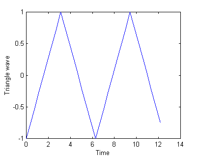
To show that this works as expected, generate a triangle wave:

» t=(0:31)*4*pi/32; %32 evenly spaced samples from 0 to 4*pi.
» z=sawtooth(t,0.5); %generate a triangle wave.
» plot(t,z)
» xlabel('Time');
» ylabel('Triangle wave');

Now lets do the analysis part where we find the frequency and amplitude of the sinusoids that make up this wave.

» dt=t(2)-t(1);             %Time step between samples.
» [mz,pz,f]=swatFFT(z,dt);  %Take the FFT.
» stem(f,mz)                %This is just another kind of plot.
» xlabel('Frequency (Hz)')
» ylabel('Amplitude')

The function swatFFT takes the FFT of the vector "z", and calculates the magnitudes ("mz") and frequencies ("f") of all the component sinusoids.  There is another quantity ("pz") which corresponds to the relative phase of all the sinusoids (in case they aren't all lined up).  Recall that in general a sine wave is given by A*sin(wt+q), i.e. it has a magnitude (A) a frequency (w) and a phase (q).

2) Print the plot you just made.  In what ways does the plot of the FFT look like you'd expect?  Is it different in any ways?  You may want to refer to last week's lab.

Sampling

Let's start again with a 200 Hz sine wave

» fs=1000;
» dt=1/fs;
» t=(0:2047)*dt;
» f=200;
» x=sin(f*2*pi*t);
» sound(x,fs)
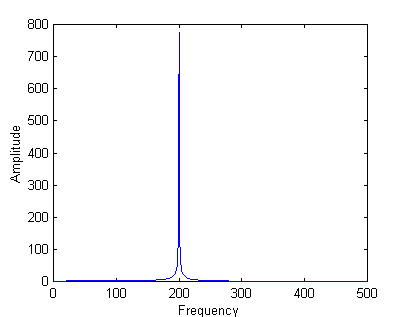
» [xm,xp,fq]=swatFFT(x,dt);
» plot(fq,xm)
» xlabel('Frequency');
» ylabel('Amplitude');

These commands produce the graph shown

which as expected shows a strong signal at 200 Hz.   Repeat for a 400 Hz signal, 600 Hz signal, 1000 Hz signal.  Make sure you also listen to your signal in each case.  You may also want to try some other frequencies.  Make note of the vertical scale in all cases.

3) Plot, print, and explain, your results for the 600 Hz and 1000 Hz signals.  The 1000 Hz signal is probably easier to explain.

Unfortunately the FFT only gives us global information about the frequency content of a waveform.  Consider a chirp signal.

» fs=1000;
» dt=1/fs;
» t=(0:2047)*dt;
» f=(0:2047)/8.192;
» x=sin(f*2*pi.*t);
» sound(x,fs)
» z=fliplr(x);        %reverse x.
» sound(z,fs)

4) Explain the relationship between the sound for the signal "x" and the signal "z".

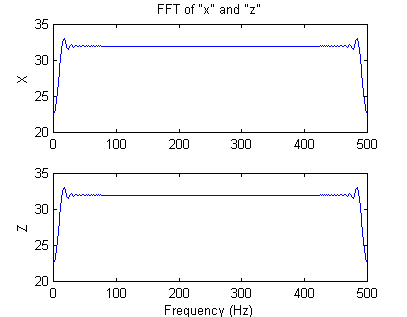
Clearly "x" and "z" are quite different, but not if we examine their FFT's.

» [xm,xp,fq]=swatFFT(x,dt);
» [zm,zp,fq]=swatFFT(z,dt);
» subplot(211);             %make two plots.
» plot(fq,xm);
» ylabel('X');
» title('FFT of "x" and "z"')
» subplot(212);             %select second plot.
» plot(fq,zm); 
» ylabel('Z');
» xlabel('Frequency (Hz)');

Note that the plots are exactly the same.  

5) How can this be?

The Spectrogram

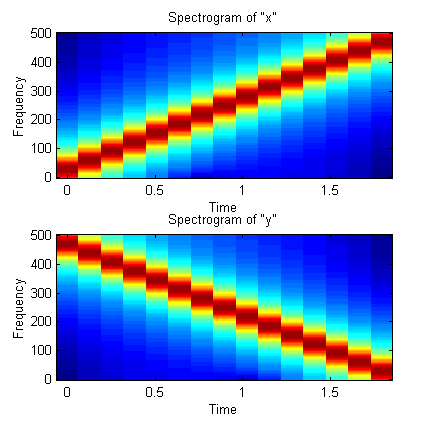
We can get both time and frequency domain information from the spectrogram.

» subplot(211)
» specgram(x,[],fs)
» title('Spectrogram of "x"');
» subplot(212)
» specgram(z,[],fs)
» title('Spectrogram of "y"');

These plots clearly show the ascending pitch of "x" and the descending pitch of "y".

Reload the music file from earlier in the lab:

» [y,fs,b]=wavread('ekn.wav');

Plot it's spectrogram. This may take some time, the vector y is large (over 500,000 elements). The vector is almost half empty (the large blank area on the spectrogram). The reasons for this are a little complex, but I'll explain it to you if you are curious.

» specgram(y,[],fs)

6) Label and print the spectrogram.

Bass and Treble Controls

Take the FFT of the sound file data.  This may take several seconds because of the length of the data set.

» [y,fs,b]=wavread('ekn.wav');  %use any sound file.
» dt=1/fs;
» [ym,yp,fq]=swatFFT(y,dt);
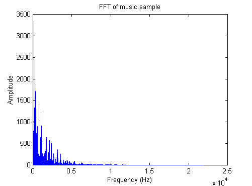
» plot(fq,ym)

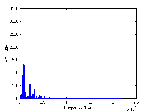
Take any sound below about 500 Hz to be in the base range, and any part above that to be treble.  Modify the signal, "ym", so that the bass part is only one tenth the amplitude of the original.   Hint: you'll probably want to use the colon operator from the last lab.

The new signal is shown below.  

Regenerate the modified time domain data by using the inverse FFT (swatIFFT), and play it.  Note that the function call here is swatIFFT, not swatFFT (the IFFT refers to the Inverse FFT):

» df=fq(2)-fq(1);
» [z,t]=swatIFFT(ym,yp,df);
» sound(z,fs)      %play modified signal
» sound(y,fs)      %play original for comparison

You should notice much less bass in the resulting signal.

7) Show the Matlab commands you used to reduce the amplitude of the bass frequencies.

8) Label and print the spectrogram of the modified signal ("z").

You could also use this technique to increase the treble part of the signal.  Or you could generalize it to several frequency bands and create a graphic equalizer.

Extra

You only need to do this if you want to - otherwise you should feel free to leave.

Generate a chirp signal.

» fs=1000;
» dt=1/fs;
» t=(0:2047)*dt;
» f=(0:2047)/8.192;
» x=sin(f*2*pi.*t);
» specgram(x,[],1000)
» sound(x,fs)

What do you expect your maximum frequency to be (try »max(f))?  What is the maximum frequency shown by the spectrogram?

9) Explain your results.  Hint, think trig identities.

Repeat with

» f=(0:2047)/4.096;
» x=sin(f*2*pi.*t);
» specgram(x,[],1000)
» sound(x,fs)

10) Explain your results.